

As many data-scientists, we often deal with the question how to extract all of the contained information from a data-set without exploding feature dimensionality while setting aside a reasonable timeframe for feature-engineering. Let’s emphasize the word „information“.
Working with time-series we most commonly think of seasonality, be it daily, weekly, or otherwise. For many human-behavior related data-sets, we expect people to keep their habits based on regular intervals. Accordingly, one would produce corresponding features (e.g. using lags of time-series) and, probably, employ smoothing to rule out random fluctuations (noise). Though, methods exist to distinguish most optimal lag-terms and, moreover, models that take care of time-series autoregressive forecasts out-of-the-box, doing so might not always bring the maximal information extraction. A certain piece of information can get lost, like for example local context influence (e.g. certain daily patterns) and/or affine transformations on the structure (i.e. rotation or inversion in terms of time, scaling with a constant, translation of particular patterns along the time line) of existing known patterns. Several model architectures exist that are capable of identifying latent features from larger input spaces, given that those possess any kind of topological structure (i.e. sequence, grid, 3-D space). In those models, feature extraction and a learning task like regression or classification are carried out subsequently as part of a single computation graph. Two main families of such algorithms are Recurrent and Convolutional neural networks. Abstracting from details and different combinations of both, the first type iterates through the data, mixing in previous iteration’s outputs, while the second type goes through the whole input with a kernel/filter/mask performing a convolution operation.
For developing a forecast model based on these algorithms, time-series non-stationarity (i.e. when the distribution on the data varies over time) and structural breaks in time-series are yet other hurdles to overcome. Those issues can be approached with additional explanatory meta-data variables, if available. These can be introduced to some computation in combination with our time-series inputs. For instance, external factors like weather and solar radiation may have great influence on what happens to energy consumption and are naturally represented as metric timeseries. Other important behavioral influences can only be explained through categorical variables like weekdays or binary variables representing holidays, bridging days and other special occasions. Such features might be able to explain non-seasonal variation inside the time series, but can also introduce a many-to-one relation, where one feature value is related to a certain subset of time-series. Uniting a whole data sequence with a sensible set of additional variables should provide the best performance, yet it is tricky to decide how to „unite“ them in an optimal way. Joining inputs horizontally brings redundancy through repetition (i.e. each external factor is supposed to be repeated along the whole length of the sequence). Vertical joining or extending the sequence will simply make a data-set inconsistent.
Another approach is to use one of the previously named neural network architectures to project the data into latent space and then concatenate it with extra variables for further computations. To do so, a projector network is built using the initial time-series data. Typically, the most common way is to train a model employing an autoencoder architecture and use an „encoder“ part of a projection model. Projected representations can then be used alongside the original data as independent variables. Though completely valid and working, this method has some unwanted properties: one must discard half of the weights of the full autoencoder after spending the necessary computation power to train them.
To rectify this situation, one could jointly train a projector and a target regressor/classifier neural network. Like in the previous suggestion, the outputs of one or more projector networks will be concatenated with other inputs and fed forward to a target network. The main advantage is that you spare some training time and adapt the weights in accordance with an end-task. However, projector networks might need more time to converge because of this sophisticated architecture. General complexity of the whole network with large amount of layers may yield vanishing or exploding gradients, and there is a lack of control of how exactly a projector network operates.
Yet, such architectures allow to stack as many projectors for as many data sources as the task requires. It brings us to a computation graph, accepting multiple heterogeneous inputs, which further will be referred to as multi-input networks. But… first things first. So, what does a “multi-input network” mean, as a matter of fact? Thinking of this concept one may build up an impression, which can be roughly visualized as follows:
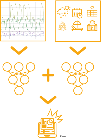
Well, frankly speaking, the reality is not quite far from what is sketched above. With the one remark, that grapes-looking conjunctions of circles and lines may represent any kind of neural networks, with the limitation that the output \(Z\) of each network is supposed to be of shape \(Z \in R^{ N_{batch} \times N_{dim}} \), i.e. the very last layer of the network is either an output of a MLP or a flattened output of a different architecture. And instead of “result” one would typically use a Concatenate (e.g. tf.keras.layers.Concatenate layer or its functional interface/alternative, depending on the computation framework you are working with. The TensorFlow (version 2) framework offers a convenient method of whole model definition for further backpropagation and gradient computation. Using tf.keras.layers.Concatenate and tf.keras.Model. Model it is possible to define a whole graph as a single function.
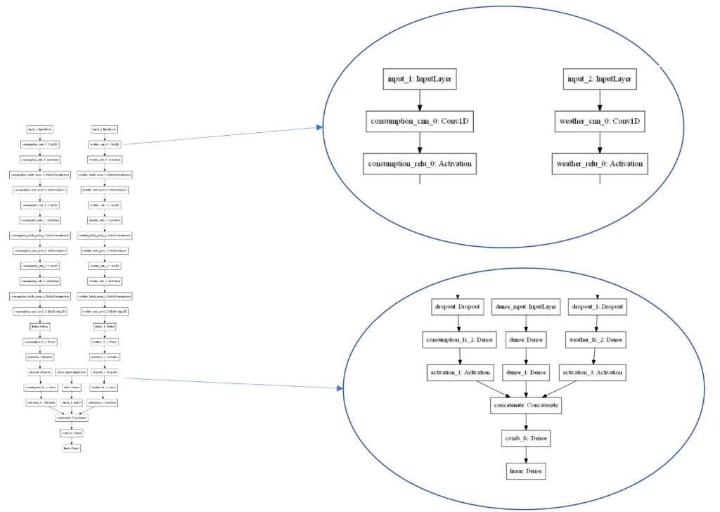
In the example below, a combined network is trained to forecast electricity consumption based on three different input sources. It receives a sequence of weather data (solar, temperature, etc.) as input1, aset of 1-dimensional features characterizing the target (e.g. Day of week, hour, month, embedded or dummy-encoded ) as input2 and, finally, a sub-sequence of electricity consumption time-series, a future element of which the network aims to predict as input3. Note, the order of individual networks, in which each part of data is processed, is completely irrelevant and can be arbitrary, whereas the choices of architecture are solely driven by the nature of each corresponding dataset. Target time-series is the input3, shifted 24 hours ahead.
Consider a snippet implementing an LSTM-based recurrent neural network for processing input1 and producing a vector of latent features of length output_dim_rnn. Given input1 is a multidimensional time-series of shape \(t \times n\) , where \(t \) is the amount of time-steps and \(n\) – amount of variables, this network is able, in an ideal scenario, to extract stationary features of shape \(1 \times h\) and reduce dimensionality, so that \(t*n≫h\).
# rnn model
model1 = Sequential()
model1.add(Input(shape=input_shape1))
return_seq = True
for i, d in enumerate(dim):
    if i == (len(dim) - 1):
        # for the last layer sequences are not required
        return_seq = False
    model1.add(LSTM(d,
                   activation=activation,
		  recurrent_activation="sigmoid",
                   recurrent_dropout=0,
                   unroll=False,
                   use_bias=True,
                   return_sequences=return_seq))
model1.add(Dense(output_dim_rnn, activation='relu'))
The following code implements a simple fully-connected network to map input2 to another set of latent features of dimensionality output_dim_rnn.
# mlp model
model2 = Sequential()
model2.add(Input(shape=input_shape2))
for d in dim:
    model2.add(Dense(d, activation=activation))
The third block is a 1D Convolutional neural network, that takes input3 (also sequential) and produces once again a set of latent features of dimensionality output_dim_cnn. The choice of architecture here is based on the data, as mentioned before.
# cnn model
model3 = Sequential()
model3.add(Input(shape=input_shape3))
for (i, f) in enumerate(filters):
    model3.add(Conv1D(f,
		     (KERNEL_SIZE[i]),
	             padding="causal", strides=strides, use_bias=False)
	      )
    model3.add(Activation("relu"))
    model3.add(BatchNormalization(axis=chanDim))
    model3.add(MaxPooling1D(pool_size=pool_size))
model3.add(Flatten())
model3.add(Dense(output_dim_cnn, activation='relu'))
Finally, all the latent features are concatenated together and passed to another fully-connected output layer. It may be beneficial to use more than one layer on top of joint latent features, this is a matter of validation and hyperparameter search. Using tf.keras.Model API it is easy to access inputs and outputs of already defined models, as well as to define a new one based on only it’s input and output.
combinedInput = concatenate([model1.output, model2.output, model3.output])
y = Dense(final_output_dim, activation=target_activation)(combinedInput)

# build final model
model = Model(inputs=[model1.input, model2.input, model3.input], outputs=y)
After the model is defined, it is straight-forward to train it with the only difference that instead of a single input, an ordered list of inputs is provided.
opt = Adam(lr=LR, decay=WD)
model.compile(loss="mean_absolute_percentage_error", optimizer=opt)
hist = model.fit(
    [x_w_train, x_ex_train, x_seq_train], y_train,
    epochs=25, batch_size=128)
Designing a multi-input neural network, one is not limited with the topology choice. Based on the application, it can as well be useful to use a concatenation operation of processed features from one network directly with new inputs.
Here is an example of how the final architecture can look like (note: the network consists of 2 CNNs and an MLP).
Weight initialization can be a game changer in such sophisticated architectures. Therefore, it is crucial to keep in mind how you handle it. Checking a selected dataset distribution and sampling initial weights of a neural network from an appropriate random distribution of weights is a good way to go. Also, pretraining individual networks will speed up convergence of a joint network.
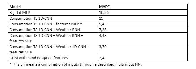
It was verified on a practical case-study with 3 years of data that this type of network architecture offers a mechanism to leverage heterogenous data structures without extensive feature-engineering. As already described, the experimental network used 3 inputs: primary electricity consumption time-series data, weather curves and different exogeneous features, analyzed respectfully by 2 CNNs and an MLP. The resulting network was able to outperform all the combinations of 2 Input- or 1 Input- networks (no surprise though, the more data – the better), as well as a big MLP with plain flattened inputs (unrolled sequences result in considerably more trainable parameters, though having same amount of layers). As an error metric – Mean Average Percentage Error was used. As a baseline and state-of-the-art for this dataset a gradient boosting model with weeks spent on feature engineering and feature selection was used.
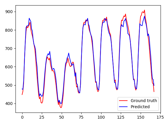
The plot below depicts one week of prediction inside the test set using the best performing combined network.
In this post we revisited the problem of tackling multiple inputs of different structure and form. While not always offering the highest prediction accuracy, multi-input or joint networks offer a lot of flexibility and adaptivity for low development cost. It doesn’t matter if one is analyzing time-series or pictures with accompanying meta-data – the mechanism is the same. The post underlines how uncomplicated it has become to build branched network architectures, using the Tensorflow v2 and previously Keras. For Proof-of-Concept, a 3-input combined network was built and benchmarked against simpler versions. The result has shown improvements for adding each sub-network for different input types accordingly. Once again, it may be not the best fit for the problem but offers acceptable results in a much smaller development time, due to zero feature-engineering and only basic data preparation efforts.